Thus, the fallacy behind drawing Figure 4 or Figure 5 is that the tolerance lines encourage us to interpret a trigonometric function as a proportion. Whenever we do this we will always be wrong.
When we understand that the P/T is a trigonometric function times a constant, we discover why this ratio is so hard to interpret.
The specified tolerance does not apply to the measurement system. Thus, any graph like Figures 4 or 5 is fundamentally flawed. These graphs encourage a bogus comparison between precision and tolerance, which can be very misleading.
Richard Lyday wanted to evaluate a new vision system used to measure the diameters of steel inserts for steering wheels. He took a single insert and measured it 30 times over the course of one hour and got the diameters shown in Figure 1.
Since this graph makes a comparison that can only be misleading, it should be ignored. The only appropriate limits for the running record of values from a Type 1 repeatability study are those of an XmR chart.
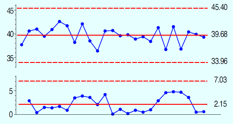
For the data of Figure 2, our estimate of the value for the known standard is 39.68 units, and our estimate for repeatability is s = 1.68 units.
Statistics
Questions About Type 1 Repeatability Studies
How to avoid some pitfalls
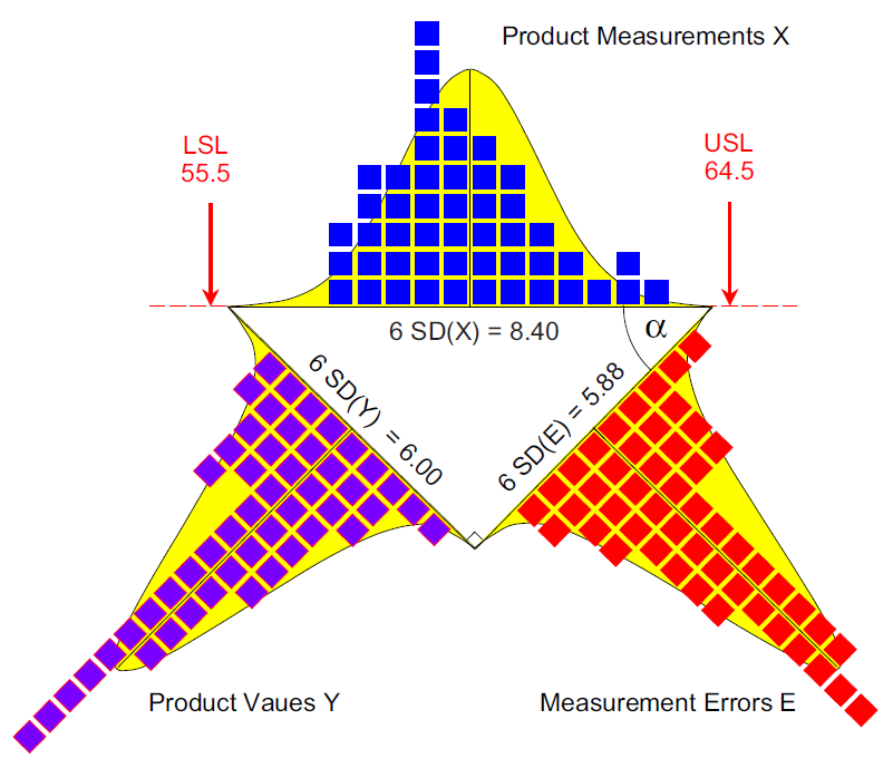
So the standard deviation of X will be the square root of 1.96, which is 1.40. Thus, the only correct way to show the relationship between the standard deviations of X, Y, and E is to use a right triangle as in Figure 8.
When the measurement process appears to be unpredictable, what do the average and standard deviation statistics represent?
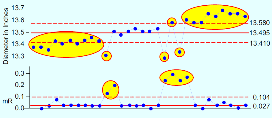
Figure 1: XmR chart for 30 measurements of the diameter of one insert
= 1.00 + 0.96 = 1.96
Consider the previous example. There we had a P/T ratio of 0.65. Based on this value, most arbitrary guidelines would condemn this measurement process. Yet here we have a process that, when operated predictably and on-target, is capable of producing essentially 100%-conforming product. Moreover, the current measurement system is adequate to allow this process to be operated up to its full potential. Here, there is no need to upgrade or change this measurement process.
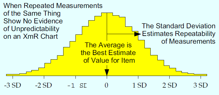
Figure 3: Descriptive statistics for a predictable measurement process
Published: Monday, August 7, 2023 – 12:04
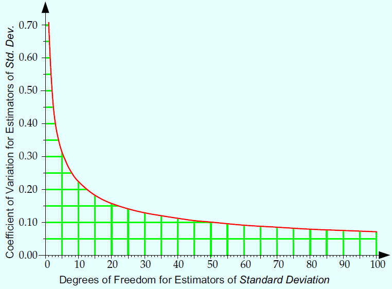
Figure 9: Uncertainty and degrees of freedom
The average for the data of Figure 1 is 13.495 in. However, since these observed values drift by 3/8 in. in the course of an hour, this average does not provide a useful estimate of the value of the measured insert. A wood yardstick would give us a more reliable measurement of the diameter of one of these inserts than is provided by this electronic vision system.
Once you pass 10 degrees of freedom, you are in the region of diminishing returns. Between 10 and 30 degrees of freedom, your estimate of repeatability will congeal and solidify. The 25 data of Figure 2 give an estimate of repeatability having a coefficient of variation of 14%. Using twice as many data would have reduced the CV to 10%. This is why, historically, Type 1 repeatability studies have been based on 25–30 data.
Question 8
In Figure 9 the vertical axis shows the coefficient of variation (CV), which is the traditional measure of uncertainty for an estimator. The coefficient of variation is the ratio of the standard deviation of an estimator to the mean of that estimator.
Since this interval includes zero, we have no detectable bias, and any bias present is likely to be less than 0.58 units. Since this is less than the probable error of 1.1 units, we can say that this test is unbiased in the neighborhood of 40.
Question 7
When a measurement process calls for multiple determinations and reports their average as the observed value, a repeatability study will require multiple determinations for each observation, with reloading between each set of multiple determinations.
Summary
Estimated probable error = 0.675 estimated SD(E)
This is why the precision-to-tolerance ratio should not be used to condemn a measurement process. It does not tell the whole story. Since money spent on measurement systems will always be overhead, we should be careful about condemning a measurement system based on a trigonometric function masquerading as a proportion.
Should we reload the part between measurements?
Yes. Sixty years ago, Churchill Eisenhart, senior research fellow and chief of the Statistical Engineering Laboratory at the National Bureau of Standards, wrote the following about Type 1 repeatability studies: “Until a measurement process has been ‘debugged’ to the extent that it has attained a state of statistical control, it cannot be regarded, in any logical sense, as measuring anything at all.”
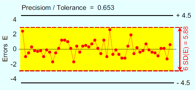
Figure 5: Measurement errors with tolerance limits added
To illustrate how the plot of the repeatabilities vs. the tolerance is misleading, I will use a synthetic example. Here we’ll assume that the specifications are 60.0 ± 4.5 units, we have a known standard with an accepted value of 60, and the measurement errors have a mean of zero and a standard deviation of 0.98. Fifty observations of this standard from a Type 1 repeatability study plotted against the specifications might look like Figure 4.
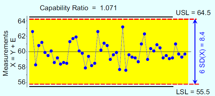
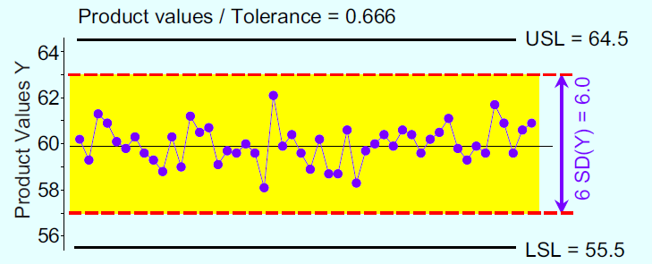
Let us now assume we have a predictable production process operating with a mean of 60 and a standard deviation of 1.00. A set of 50 product values plotted against the specifications might look like Figure 6.
Why do the simple ratios of Figures 5 and 6 not work as proportions? It has to do with a fundamental property of random variables. Whenever we plot a histogram or a running record, the variation shown will always be a function of the standard deviation. This is not a problem when we are working with a single variable, but when we start combining variables the bogus comparisons creep in because the standard deviations do not add up.
In Figure 4, we see the repeated measurements, (60+E), and the horizontal band shown is (6 SD(E)) wide. This part of Figure 4 is correct. It is the inclusion of the specifications on Figure 4 that creates a bogus comparison.
For Figure 2, the average is 0.32 units smaller than the accepted value of 40. With 24 d.f. the student-t critical value is 1.711, which gives a 90% interval estimate for the difference of:
Did Richard Lyday need additional data in Figure 1 to know that he had a rubber ruler? Without a predictable measurement process there is no magic number of readings. Without predictability, there is no repeatability and no bias. So we cannot estimate these quantities regardless of how many data we collect.
Before we can talk about bias, we have to have a predictable measurement process.
The probable error characterizes the median error of a measurement. A measurement will err by this amount or more at least half the time. As such, the probable error defines the essential resolution of a measurement and tells us how many digits should be recorded. (We will want our measurement increment to be about the same size as the probable error.)
How can a production process that consumes 67% of the tolerance be combined with a measurement system that consumes 65% of the tolerance and end up with a stream of product measurements that only use 93% of the tolerance?
All bias is relative. If we perform our Type 1 repeatability study using a known standard that has an accepted value based on some master measurement method, and if our measurements do not display a lack of predictability, then we can compare our average value with the accepted value for the standard.
No, we cannot.
A Type 1 repeatability study starts with a “standard” item. This standard may be a known standard with an accepted value determined by some master measurement method, or it may be an item designated for use with the study (an “unknown standard”). The standard is measured repeatedly, within a short period of time, by a single operator using a single instrument. Finally, these repeated measurements are used to compute the average and standard deviation statistics, and these are used to characterize the measurement process. This technique can be traced as far back as Friederich Wilhelm Bessel and his Fundamenta Astronomiae, published in 1818.
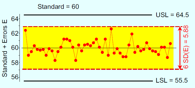
Figure 4: 50 measurements of a standard with specifications added
Thus, to cut the uncertainty in half you will have to collect four times as many observations.
With a predictable measurement process, the average statistic is your measurement system’s best estimate of the value of the measured item. When a known standard is used, the average will let you test for bias.
Do we always need to use 50 measurements?
Nothing whatsoever.
Thus, if we are not careful to compare apples with apples, bogus proportions can creep in when we work with multiple variables. While the graphs will show variation as a function of the standard deviations, these standard deviations will never be additive. This complicates comparisons among the multiple variables.
Descriptive statistics can only describe the data. Meaning has to come from the context for the data. When the data are an incoherent collection of different values, the statistics will not represent any underlying properties or characteristics.
How can you measure a part without loading it? Preparing an item for testing is part of the measurement process. Variation in preparation can contribute to measurement error. Even if parts are loaded automatically, loading the item is part of obtaining the measurement.
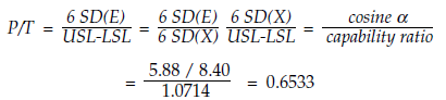
Specifications always apply to the product measurements, X. Thus the specifications, and the specified tolerance, belong on the hypotenuse of the right triangle as shown in Figure 8.
Thus, the P/T ratio is always a trigonometric function divided by the capability ratio. And everyone who has had high school trigonometry knows that we cannot treat trigonometric functions like they are proportions. They simply do not add up. Never have, never will.
When we put these two results together, we find that the precision to tolerance ratio is, and always has been:
For Figure 2, our estimate of probable error is 0.675 (1.68) = 1.1 units. This means that these measurements are good to the nearest whole number of units. They will err by 1.1 units or more at least half the time. Thus, the results for Test Method 65 should be rounded to the nearest whole number; recording fractions of a unit will be excessive.
Question 3
With a predictable measurement process, the standard deviation statistic is an estimate of the repeatability of your measurement system. This is the state of affairs shown in Figure 3.
Our predictable measurement process may be said to be biased relative to the master measurement method if and only if we find a detectable difference between the average and the accepted value for the standard. Here, we typically use the traditional t-test for a mean value. With a detectable bias, the best estimate for that bias will be the difference between the average and the accepted value.
With a predictable measurement process, the relationship between the uncertainty in an estimate of dispersion and the amount of data is shown in Figure 9.
The repeated measurements of a Type 1 repeatability study belong on an XmR chart. The notions of repeatability and bias are predicated upon having a predictable measurement process. This is why the analysis of data from a Type 1 repeatability study should always start with an XmR chart.
The standard deviation statistic of 0.114 in. for Figure 1 does not tell us anything useful about the precision of this vision system, since it has been inflated by both the trend and the upsets.
Thanks,
Quality Digest