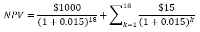
SVB invested in 10-year Treasury notes before the Federal Reserve began to raise interest rates sharply to fend off inflation.3 The SEC reference provides two examples we can use to illustrate net present value calculations. The first example is as follows:
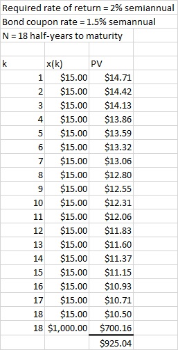
Now suppose instead that the interest rate rises from 3% to 4% for this bond. The required semiannual rate of return is therefore 2%. The SEC says the bond is worth only $925; that is, we’ve just lost $75 on a purportedly secure investment. The investment is secure in the sense that, if we wait nine years, we will collect the principal. The face value of the bond is exactly what it says nine years from now, but the bond is worth only $925 today—and this is what happened when SVB needed money quickly to pay depositors. Figure 3 shows the effect of the higher required rate of return when, for example, the second payment is divided by (1+0.02) squared rather than (1+0.015) squared for the original (3%) interest rate.
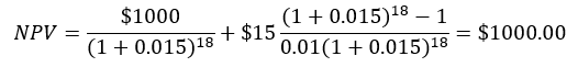
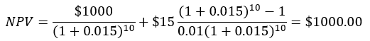
Excel will do the entire problem for us if we include the semiannual interest payments and also the bond’s redemption in the last period: =PV(0.015,18,–15,–1000) = $1,000.00. This means we can, given 1) the required rate of return; 2) the remaining periods to maturity; and 3) the semiannual coupon payment, get the current price of a bond with a single function.
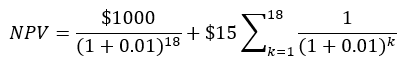
In this case, there are 18 semiannual periods remaining, each of which has a coupon payment of $15, and the bond’s principal is redeemed at the end of the last period. There is no activity (such as an investment) in period 0. Note that the required semiannual rate of return is half the required annual rate of return (2%), so we use 0.01 for i.
We can calculate this as shown in equation 1, where the required rate of return is i, there are N periods of activity, and xk is the cash flow in period k. The reciprocal of (1+i) to the kth power is the present worth factor for a single payment.1 We can, in fact, use equation 1 in spreadsheet form to solve most if not all present-worth problems.
2. =PMT(i,N,P) is the capital recovery function for a principal of P, to be paid off at interest rate i in N periods.
Lean
Introduction to Time Value of Money
These concepts play a central role in many practical and vital applications
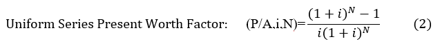
This is not particularly suitable for a calculator—who wants to do 18 successive calculations for the coupon payments?—but there is also a present worth factor for a uniform series as shown by equation 2. (P/A,i,N) is shorthand for Present worth given an Annual (or other periodic payment) with a required rate of return i, for N periods.
Financial talk show host Dave Ramsey warns that car dealers take advantage of customers by talking about payments rather than the price of the car.4 “When a salesman pops the question, ‘What kind of payment are you looking for?’ before you’ve even talked about the price of the car, that’s a major red flag.” The problem can be phrased in two ways. If the monthly payment and interest rate are known, the car’s actual price is the NPV of the uniform series. If the price and the payments are known, the interest rate can be calculated.
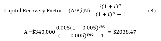
Bankrate5 has an online mortgage payment calculator. Suppose we buy a $425,000 house with a 30-year loan, a 6% interest rate, and an $85,000 down payment. This leaves a $340,000 principal that must be paid off with monthly payments. Bankrate comes up with $2,038 a month (this doesn’t count property taxes and other expenses). We can reproduce these results with the capital recovery factor for a uniform series of payments, which returns the annual (or, in this case, monthly) payment whose net present value is the principal. Equation 3 is the capital recovery factor. The monthly interest rate is 0.5% and there are 360 payments.
Excel’s NPV function can also be used, but with a caveat: It doesn’t treat the transaction in the first row as at time zero. That is, it will divide the ($100,000) payment by (1+0.15) and the subsequent $18,000 after tax income by (1+0.15) squared. Microsoft explains on its website, emphasis is mine:
3. =NPV(i,x1,x2,…,xN) returns the net present value of a series of N payments and/or receipts, given a required rate of return i, but assumes they take place at the end of each period. That is, the first transaction is discounted by 1/(1+i).
=PV(0.02,18,–15,–1000) returns the same result of $925.04. This is the most convenient way to do this problem in Excel; the tabulations are useful primarily for illustrating the effect of time on the present value of the money. Note that the present value of the bond redemption is only $700.16 rather than $764.91, the present worth if the required semiannual rate of return is 1.5%. This is the source of most of the damage ($64.75) because the biggest amount involved, $1,000, is paid farthest out, where it is divided by (1+0.02) to the 18th power.
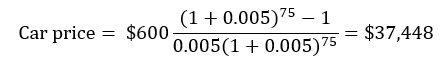
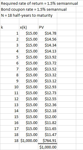
Figure 1: Calculation of bond value, 1.5% semiannual required rate of return
We will see that Excel also has a function for net present value, but it requires the income and expenditures to be in separate cells, with one cell per time period. If we wanted to use it on the information in figure 1, we would have to combine the last coupon payment with the bond’s redemption value because the function would otherwise treat the redemption value as taking place in the 19th period. The NPV function will be demonstrated later on.
Effect of interest rate changes on bond values
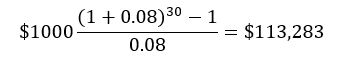
The series compound amount factor (equation 4) returns the future amount from an annual or other periodic investment, given an interest rate or other rate of return i. This illustrates the benefit of regular investments in a 401k or Roth retirement plan.
“When the U.S. government guarantees a bond, it guarantees that it will make interest payments on the bond on time and that it will pay the principal in full when the bond matures. There is a misconception that, if a bond is insured or is a U.S. government obligation, the bond will not lose value. In fact, the U.S. government does not guarantee the market price or value of the bond if you sell the bond before it matures. This is because the market price or value of the bond can change over time based on several factors, including market interest rates.”
This article has also covered some useful Excel functions.
1. =PV(i,N,A,(F)), where i is the required rate of return, N the number of periods, A the periodic payment, and F, an optional lump sum payment at the end of the series, can calculate the present value of a bond. The function assumes we are paying money, so we must use negative numbers for A and F if we are receiving payments.
• PV(i,N,A) is the function for the present worth of a uniform series.
• PV(i,N,0,F) is the present worth of a single future amount.
Suppose we pay $1,000 for a 10-year Treasury note with an annual interest of 3%. The bond pays interest semiannually at 1.5%, so the coupon payment is $15. If the required rate of return on our investment is 3%, the net present value (NPV) of the bond is $1,000 regardless of the remaining time to maturity. This is because the discounted cash flows of the interest payments and the bond’s face value at redemption always equal $1,000 as long as the available interest rate for similar bonds doesn’t change.
SVB invested in 10-year Treasury notes when the interest rates were even lower; let’s say 1.5% as an example. I saw a 3.5% rate quoted around March 2023, so let’s see what happens if there were eight years left to maturity for SVB’s notes. Also assume 3.5% applies to eight-year notes. There are 16 semiannual periods left, the required semiannual rate of return is 1.75%, and the coupon payment is $7.50. The results aren’t pretty. =PV(0.0175,16,–7.5,–1000) returns $861.50, i.e., if the bonds must be sold immediately, each will incur a $148.50 (14.85%) loss on the principal.
Car payments

The remaining time to maturity is irrelevant if the available interest rate remains unchanged. Assume that the bond now has five years (10 semiannual periods) left to maturity. The NPV is still $1,000 because, even though fewer coupon payments remain, the principal is closer to repayment, so it is discounted by (1+0.015) to the 10th power rather than the 18th power.
Time value of money calculations play a central role in many practical and vital applications. These include awareness and quantification of the effects of prevailing interest rates and time to maturity of bonds, which played a central role in the failure of Silicon Valley Bank. They are useful in the assessing mortgages and car payments, including revealing the actual cost of a car loan in contrast to what the dealer might tell us. Among their key workplace applications is assessment of projects and investments to determine whether they meet the company’s required rate of return. While the subject is beyond the scope of this article, multiple projects or proposals can be compared in this manner to obtain the best possible allotment of limited resources.
Time value of money calculations, including net present value analysis, is important when selecting projects and investments. The calculations are part of the body of knowledge for some of ASQ’s certification exams. They also go a long way toward explaining exactly what happened to Silicon Valley Bank (SVB) just a couple of months ago.
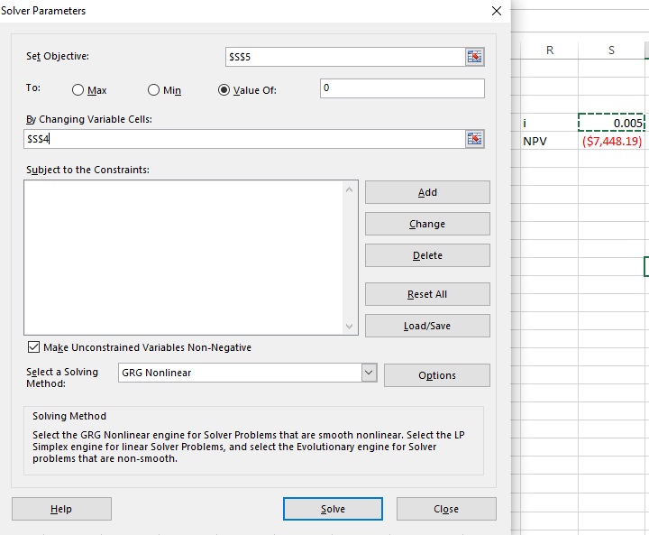
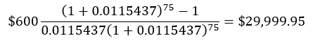
Now suppose the car’s sticker price is $30,000, and the dealer quotes 75 easy payments of $600. We can use Excel’s Solver function to find the internal rate of return (IRR) that returns a net present value of zero. That is,
References
1. Rigg, James. L. Engineering Economics. McGraw-Hill College, 1977. This book is an excellent reference for time value of money.
2. SEC’s Office of Investor Education and Advocacy. “Interest Rate Risk—When Interest Rates Go Up, Prices of Fixed-Rate Bonds Fall.” Public domain.
3. Vanek Smith, Stacey. “Bank fail: How rising interest rates paved the way for Silicon Valley Bank’s collapse.” NPR, March 2023.
4. Ramsey Solutions. “6 Tactics of a Used Car Salesman.” Website, Oct. 2022.
5. Bankrate. Mortgage Calculator.
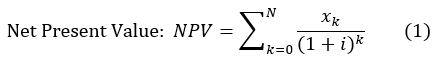
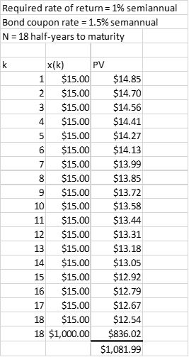
Figure 2: Calculation of bond value, 1% required semiannual rate of return
The results appear in Figure 2, and Excel’s PV function returns the same result: =PV(0.01,18,-15,-1000) = $1081.99. Remember that this function assumes positive numbers to be payments, so we must use negative values for income.
Excel’s IRR function also can be used, but it’s apparently necessary to have 76 rows; one with the +$30,000 at time zero, followed by 75 cells with negative 600 for the payments. This also returns 0.0115437.
Calculation of mortgage payments
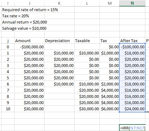
Net present value is a generally accepted way to determine whether a project or investment meets the requirements of the business, again given a required rate of return. The model can account for the effects of taxes and depreciation as well. Suppose a proposed investment of $100,000 will return $20,000 a year for 10 years, after which the relatively obsolete capital item can be sold for $10,000. This is known as its salvage value. Depreciation is over five years, with the 10-20-20-20-20-10 method, and the tax rate is 20%. The organization requires a 15% return on its investments. Figure 5 shows that this problem can be handled relatively easily on a spreadsheet.
Many SVB depositors didn’t invest in certificates of deposit but used their accounts instead to collect receivables and pay expenses and obligations, such as wages. When those depositors needed their money, SVB couldn’t come up with it. The bank looked to other assets, such as its 10-year Treasury notes with principal guaranteed by the federal government, only to find that this relates to the distant future rather than right now. The U.S. Securities and Exchange Commission (SEC) warns (emphasis is mine):2
Our PROMISE: Quality Digest only displays static ads that never overlay or cover up content. They never get in your way. They are there for you to read, or not.
The PV function will also return the present value of a single future payment, in this case the bond’s face value; =PV(0.015,18,0,–1000) returns $764.91, noting that the last argument is the optional one for the future value.
4. =IRR(x0,x1,…,xN) returns the internal rate of return for a series of N+1 payments and/or receipts; in this case, the first value (such as an initial investment) is treated as happening at time zero and isn’t discounted.
The net present value (NPV) of a project or investment is simply the sum of the positive and negative discounted cash flows throughout its life. Bonds are a good way to illustrate this concept, but we can move on to apply it to project evaluation. If, for example, a company requires a 15% rate of return on its investments, and we can estimate a future income stream, we can determine whether a proposal will meet or exceed this requirement.
Net present value of a bond
• A 10-year bond with a 3% coupon rate (the same one we used in the prior example when the required rate of return did not change) is purchased for $1,000. Interest payments are semiannual and are not reinvested. This means the bond pays $15 every half-year.
• The interest rate for nine-year bonds falls to 2% the following year. That is, if we invest money in a bond with nine years left to maturity, we can get only 2%, or a semiannual coupon payment of $10, for it. Our bond pays 3%, which makes it more valuable to investors; the SEC quantifies this as $1,082. If we’ve held the bond more than a year, we can sell it for an $82 long-term capital gain. The reference doesn’t say how it got this value, but we can use what we already know to reproduce these results.
Excel has a built-in function called PMT for the capital recovery factor. The arguments are 1) the interest rate; 2) the number of periods; and 3) the present value of the principal. =PMT(0.005,360,340000) returns $2038.47 in red, which means it is a payment rather than income. This function can also return a monthly car loan payment, given the interest rate, number of payments, and price of the car (or price minus down payment).
Assessment of a project or investment
Suppose there are nine years left to maturity, and therefore 18 semiannual coupon payments along with redeeming the bond’s face value in the last period. There is no activity (such as an investment) in period 0. Note that the required semiannual rate of return is half the required annual rate of return (3%).
Published: Tuesday, June 13, 2023 – 12:03
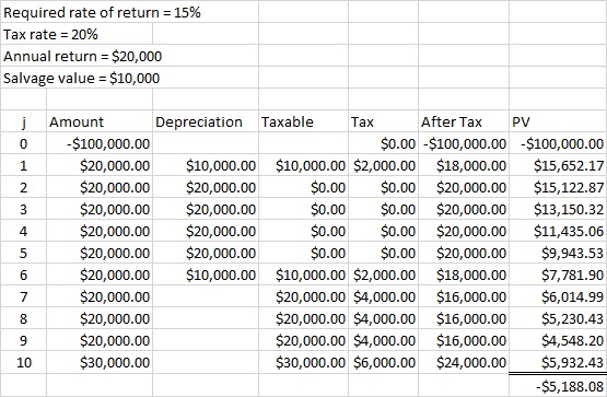
Figure 5: Assessment of an investment
Treasury bills, bonds, and notes (all similar except in terms of time to maturity) offer a simple illustration of the basic idea. The federal government takes your present money, say, $1,000, and agrees to return it at the bond’s maturity. Future money has a lower present worth than present money, so the government pays interest for its use.
Quality Digest