If the tail gets both elongated and thinner at the same time, something has to get stretched. To visualize what gets stretched, we’ll look at the radii for intervals centered on the mean that contain a specified area under the curve. The columns in Figure 6 show different specified areas, while the rows correspond to different Weibull distributions.
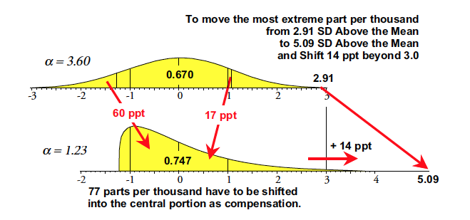
Figure 4: How the tails get lighter with skewness for Weibull distributions
The second unexpected characteristic of the Weibulls is seen in the top curve of Figure 3, which shows the areas within three standard deviations of the mean. While these areas do drop slightly at first, they stabilize for the J-shaped Weibulls at about 98%. This means that a fixed-width, three-standard-deviation central interval for a Weibull distribution will always contain approximately 98% or more of that distribution.
Figure 3 plots the areas within one, two, and three standard deviations of the mean for Weibulls with positive skewness. The bottom curve of Figure 3 (k = 1) shows that the areas found within one standard deviation of the mean of a Weibull distribution will increase with increasing skewness. Since the tails of a probability model are traditionally defined as those regions that are more than one standard deviation away from the mean, the bottom curve of Figure 3 shows us that the areas in the tails must decrease with increasing skewness. This contradicts the common notion about skewness being associated with a heavy tail.
The purpose of analysis is insight. To gain insight we have to detect any potential signals within the data. To detect potential signals we have to filter out the probable noise. And filtering out the probable noise is the objective of statistical analysis.
However, someone has to pay for this content. And that’s where advertising comes in. Most people consider ads a nuisance, but they do serve a useful function besides allowing media companies to stay afloat. They keep you aware of new products and services relevant to your industry. All ads in Quality Digest apply directly to products and services that most of our readers need. You won’t see automobile or health supplement ads.

So, while skewness is associated with one tail being elongated, that elongation doesn’t result in a heavier tail but rather in a lighter one. Moreover, Figure 3 also contains a couple of additional surprises about this family of distributions. The first of these is the middle curve (k = 2), which shows the areas within two standard deviations of the mean. The flatness of this curve shows that the areas within two standard deviations of the mean of a Weibull stay at about 95% to 96% regardless of the skewness.

and the variance of a Weibull distribution is

For example, the J-shaped Weibull model with an alpha parameter of 1.000 will have 92% of its area within 1.52 standard deviations of the mean, and it will have 98% of its area within 2.91 standard deviations of the mean.
where the symbol Γ(Α) denotes the gamma function (for A > 0):
Figure 8 summarizes how this approach works with lognormals, gammas, and Weibulls. As long as our processes are subject to signals that have an economic impact, we need not be concerned with the exact risk of a false alarm. We collect data to take action when appropriate. The one-size-fits-all approach of three-sigma limits is sufficiently conservative to minimize the risk of false alarms while allowing us to detect signals of economic importance, and they do this regardless of the shape of the histogram.
So please consider turning off your ad blocker for our site.
Quality Digest does not charge readers for its content. We believe that industry news is important for you to do your job, and Quality Digest supports businesses of all types.
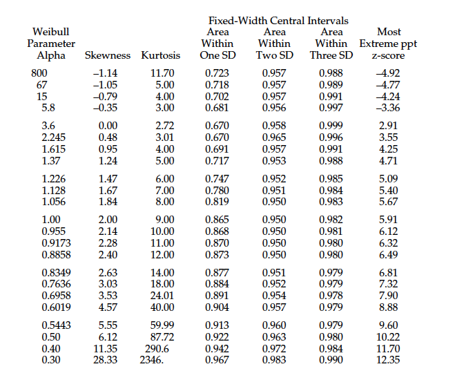
Figure 2: Characteristics for various Weibull models
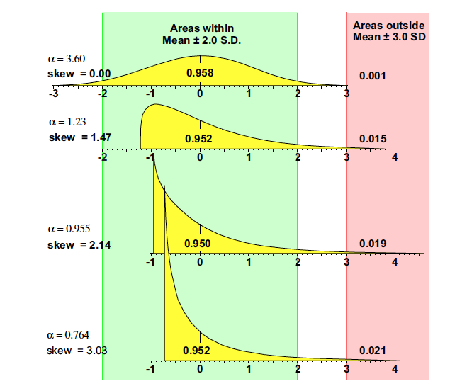
Figure 5: What Weibull distributions have in common
So what gets stretched?
The z-scores for the last part per thousand in Figure 2 show that the upper tails become elongated with increasing positive skewness. But there is a surprise contained in the other columns of Figure 2.
Thanks,
Quality Digest
منبع: https://www.qualitydigest.com/inside/lean-article/what-you-need-know-about-weibull-distributions-030624.html
This approach, where you specify the amount of noise to be filtered out, is equivalent to using the table in Figure 6. So, here you fit a model, choose a specific area to filter out, and then find the exact width of interval to use in packaging the noise. (Unfortunately, the apparent precision of this approach is offset by the uncertainty inherent in fitting a specific model to the data.)
Over the past two months we’ve considered the properties of lognormal and gamma probability models. Both of these families contain the normal distribution as a limit. To complete our survey of widely used probability models, this column will look at Weibull distributions, a family that doesn’t contain the normal. As before, an appreciation of the properties of Weibull distributions will allow you to obtain results that are reliable, solid, and correct while avoiding the pitfalls of overly complex analyses.
The Weibull distributions
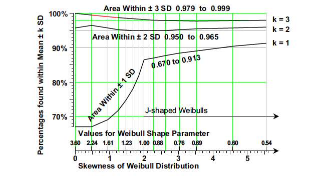
Figure 3: How the coverages vary with skewness for Weibull distributions
So, what is changing as you select different Weibull probability models? To answer this question, Figure 2 considers 23 different Weibull models. For each model we have the skewness and kurtosis; the areas within one, two, and three standard deviations on either side of the mean; and the z-score for the most extreme part per thousand of the model.
The alpha parameter determines the shape of the Weibull distribution, while the beta parameter determines the scale. Since we’ll consider the Weibulls in standardized form, where the distribution is shifted to have a mean of zero and stretched or shrunk to have a standard deviation of 1.00, the value for the beta parameter won’t matter. Changing the value of beta will not affect any of the results noted here. Thus, the horizontal scale for the probability models shown in the figures that follow are in standard deviation units.

The mean of a Weibull distribution is
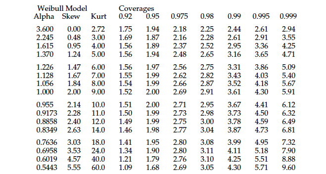
Figure 6: Radii for central intervals covering fixed areas
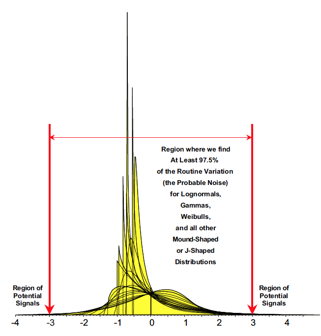
Figure 8: Three-sigma limits for lognormals, gammas, and Weibulls
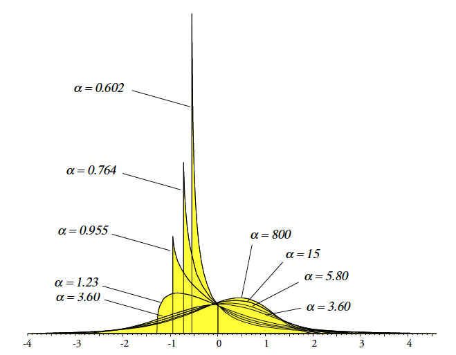
Figure 1: Eight standardized Weibull distributions
Lean
What You Need to Know About Weibull Distributions
The more you know, the easier it becomes to use your data
Fortunately, by understanding the properties of probability models, a simpler approach is possible. Once we realize that virtually all mound-shaped and J-shaped probability models will have 98% to 99.9% within three standard deviations of the mean, we no longer need to laboriously fit a particular probability model to our data. We can use three-sigma limits centered on the average to filter out virtually all of the routine variation, and treat anything left over as a potential signal.
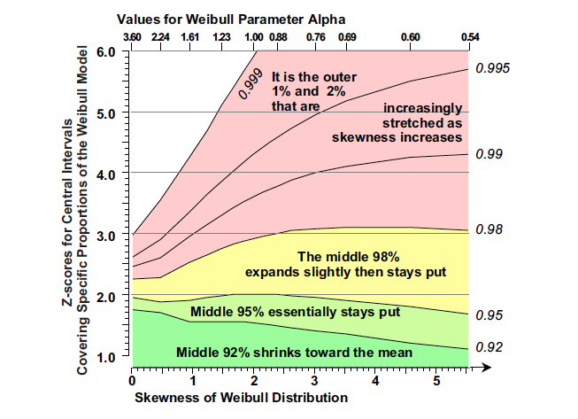
Figure 7: Widths of fixed-coverage central intervals for Weibull models
Theoretical models such as the lognormals, gammas, and Weibulls may be used to develop methods of analysis that will allow us to filter out some specified amount (usually 95%) of the probable noise. Anything left over after we filter out the bulk of the noise is a potential signal.
The spread of the top three curves shows that for the Weibull models it’s primarily the outermost 2% that gets stretched into the extreme upper tail. Although 920 parts per thousand are moving toward the mean, and another 60 parts per thousand get slightly shifted outward and then stabilize, it’s primarily the outer 20 parts per thousand that bear the brunt of the stretching and elongation that goes with increasing skewness.
The purpose of analysis
When the alpha parameter is 1.00 or less, the Weibull model will be J-shaped. When the alpha parameter is between 1.00 and 3.60, the Weibull distributions will be mound-shaped with positive skewness. When the alpha parameter is greater than 3.60, the Weibull models will be mound-shaped and negatively skewed. Since the shape of these negatively skewed Weibull models essentially stops changing as the alpha parameter increases beyond 10.0, the negatively skewed Weibulls are of little practical interest. This freezing in shape can be seen by comparing the standardized distributions for a = 15 and a = 800 in Figure 1.
Weibull distributions are widely used in reliability theory and generally found in most statistical software packages. This makes these distributions easy to use without having to work with complicated equations. The following equations are included here in the interest of clarity of notation. The Weibull distributions depend upon two parameters, denoted here by alpha and beta. The cumulative distribution function for the Weibull family has the form:
Each column in Figure 6 is used to create a curve in Figure 7 by plotting the radii in a column vs. their skewness values. The bottom curve shows that the middle 92% of a Weibull will shrink with increasing skewness. The 95% fixed-coverage intervals are remarkably stable until the increasing mass near the mean eventually begins to pull this curve down. The 98% fixed-coverage intervals initially grow, and then they plateau near three standard deviations.
Published: Wednesday, March 6, 2024 – 12:03